Lecture 11 (4/20/2022) — UCSD CSS 2

What is wide data?¶

…

When we interact with data that’s made to be read by people, it’s most often in wide format.

The definition of wide data can be a little hard to pin down but one rule of thumb is that wide data spreads multiple observations or variables across columns in a given row.

y	x1	x2	x3
1	a	b	c
2	d	e	f
…	…	…	…

Here’s some data I made up about average temperatures in five US cities over three consecutive years:

cities = pd.DataFrame({
    "City": ["San Diego", "Denver", "New York City", "Los Angeles", "San Francisco"],
    "2010": [75, 60, 55, 65, 70],
    "2011": [77, 63, 58, 67, 72],
    "2012": [77, 62, 56, 67, 71]
})

cities

	City	2010	2011	2012
0	San Diego	75	77	77
1	Denver	60	63	62
2	New York City	55	58	56
3	Los Angeles	65	67	67
4	San Francisco	70	72	71

This data can also be presented with year as our variable of interest and each city as a column:

years = pd.DataFrame({
    "Year": [2010, 2011, 2012],
    "San Diego": [75, 77, 77],
    "Denver": [60, 63, 62],
    "New York City": [55, 58, 56],
    "Los Angeles": [65, 67, 67],
    "San Francisco": [70, 72, 71]
})

years

	Year	San Diego	Denver	New York City	Los Angeles	San Francisco
0	2010	75	60	55	65	70
1	2011	77	63	58	67	72
2	2012	77	62	56	67	71

Both of these are pretty easy to read and pretty intuitive.

What kind of questions can we answer most easily with each dataframe?

cities: how do the cities differ in their temperatures?

years: which year was the warmest?

Note: this is easiest to illustrate with time sequence data, but most data can be toggled around this way to some degree:

students = pd.DataFrame({
    "Student": ["Erik", "Amanda", "Maia"],
    "Math": [90, 95, 80],
    "Writing": [90, 85, 95]
})

students

	Student	Math	Writing
0	Erik	90	90
1	Amanda	95	85
2	Maia	80	95

classes = pd.DataFrame({
    "Subject": ["Math", "Writing"],
    "Erik": [80, 95],
    "Amanda": [95, 85],
    "Maia": [80, 95]
})

classes

	Subject	Erik	Amanda	Maia
0	Math	80	95	80
1	Writing	95	85	95

The first table makes it easier to ask questions like “which student performed best?”, while the second is easier for asking questions like “are these students better at math or writing?”

Self-quiz: do the above examples give you an okay intuition for what wide data looks like?

So what’s the problem?¶

First, the exercise above suggests that for different kinds of questions, we need to format our data in different ways. That seems onerous…
Second, even though tables like this make these data easy to read as humans, answering questions about the data when it’s formatted like this can be difficult and inefficient.

Using the data below, how do we figure out which city was hottest on average (using our python skills)?

cities

	City	2010	2011	2012
0	San Diego	75	77	77
1	Denver	60	63	62
2	New York City	55	58	56
3	Los Angeles	65	67	67
4	San Francisco	70	72	71

# CODE HERE
cities
# for loop over rows and compute value

cities = cities.assign(avg = lambda row: np.mean(row[['2010', '2011', '2012']], axis = 1))
cities

	City	2010	2011	2012	avg
0	San Diego	75	77	77	76.333333
1	Denver	60	63	62	61.666667
2	New York City	55	58	56	56.333333
3	Los Angeles	65	67	67	66.333333
4	San Francisco	70	72	71	71.000000

Notice that we have to do this by calculating an average row by row. Seems inefficient.

Can we do any better with our years dataframe?

years

	Year	San Diego	Denver	New York City	Los Angeles	San Francisco
0	2010	75	60	55	65	70
1	2011	77	63	58	67	72
2	2012	77	62	56	67	71

# CODE HERE

# ???

Using the data below, how do we decide which year had the highest recorded temperature across these cities?

years

	Year	San Diego	Denver	New York City	Los Angeles	San Francisco
0	2010	75	60	55	65	70
1	2011	77	63	58	67	72
2	2012	77	62	56	67	71

# CODE HERE

years = years.assign(temp = lambda row: np.mean(row[['San Diego', 'Los Angeles']], axis = 1))
years

	Year	San Diego	Denver	New York City	Los Angeles	San Francisco	temp
0	2010	75	60	55	65	70	70.0
1	2011	77	63	58	67	72	72.0
2	2012	77	62	56	67	71	72.0

Yikes 😬

Self-quiz: is it clear how data that’s easy to read in wide format can be kind of tricky to interact with when trying to analyze it in python?

What do we do about this? Answer: tidy (long) data!¶

With long or tidy data, every observation gets its own row, with columns indicating the variable values that correpond to that observation.

The wide table at the beginning of the previous section looked like this:

y	x1	x2	x3
1	a	b	c
2	d	e	f
…	…	…	…

Compare the table above to this one:

y	variable	value
1	x1	a
1	x2	b
1	x3	c
2	x1	d
2	x2	e
2	x3	f
…	…	…

Here’s a concrete example with the student data above.

In wide form, it looked like this:

students

	Student	Math	Writing
0	Erik	90	90
1	Amanda	95	85
2	Maia	80	95

In tidy form, it looks like this:

tidy_students = pd.DataFrame({
    "Student": ["Erik", "Erik", "Amanda", "Amanda", "Maia", "Maia"],
    "Subject": ["Math", "Writing", "Math", "Writing", "Math", "Writing"],
    "Score": [90, 90, 95, 85, 80, 95]
})

tidy_students

	Student	Subject	Score
0	Erik	Math	90
1	Erik	Writing	90
2	Amanda	Math	95
3	Amanda	Writing	85
4	Maia	Math	80
5	Maia	Writing	95

Self-quiz: is it clear how the tidy data here differs from wide data?

If you want to go into the weeds on this, here’s a paper by the inventor of tidyverse, a large library in R with many similar functions to pandas.

So what does tidy data do for us?¶

The tidy data in the previous examples are harder to read and harder to interpret in the ways we often want to think about tabular data.

So how does this help us?

Summary

Tidy data avoids the pitfalls of having to reformat our data for different kinds of questions (usually)
Tidy data enforces structure so there isn’t confusion about how best to represent our data (there may be multiple wide formats but usually only one tidy format) -> best practice
Tidy data is easier to interact with and analyze with code
Tidy data lets us take advantage of the vectorization that numpy, pandas, and other modern coding languages employ to make calculations super speedy

Example

Let’s go through a simple example with the temperature data above.

Here’s the original wide dataframe:

cities

	City	2010	2011	2012	avg
0	San Diego	75	77	77	76.333333
1	Denver	60	63	62	61.666667
2	New York City	55	58	56	56.333333
3	Los Angeles	65	67	67	66.333333
4	San Francisco	70	72	71	71.000000

Here it is in tidy format:

tidy_cities = pd.DataFrame({
    "City": ["San Diego", "San Diego", "San Diego", 
             "Denver", "Denver", "Denver", 
             "New York City", "New York City", "New York City", 
             "Los Angeles", "Los Angeles", "Los Angeles", 
             "San Francisco", "San Francisco", "San Francisco"
            ],
    "Year": [2010, 2011, 2012, 
             2010, 2011, 2012, 
             2010, 2011, 2012, 
             2010, 2011, 2012, 
             2010, 2011, 2012
            ],
    "Temp": [75, 77, 77,
             60, 63, 62,
             55, 58, 56,
             65, 67, 67,
             70, 72, 71
            ]
})

tidy_cities

	City	Year	Temp
0	San Diego	2010	75
1	San Diego	2011	77
2	San Diego	2012	77
3	Denver	2010	60
4	Denver	2011	63
5	Denver	2012	62
6	New York City	2010	55
7	New York City	2011	58
8	New York City	2012	56
9	Los Angeles	2010	65
10	Los Angeles	2011	67
11	Los Angeles	2012	67
12	San Francisco	2010	70
13	San Francisco	2011	72
14	San Francisco	2012	71

Now, let’s return to our original question: which city was the hottest on average during this time?

# CODE HERE

tidy_cities.groupby(
    ['City']
).agg(
    city_avg = ('Temp', 'mean')
).reset_index(
).nlargest(
    1, 
    'city_avg'
)

	City	city_avg
3	San Diego	76.333333

That was pretty easy.

And under the hood, pandas groupby means that we compute the average temperature using vectorization rather than calculating row by row as we did in the solution above.

What about our second question: which year had the highest recorded temperature?

# CODE HERE

tidy_cities.groupby(
    ['Year']
).agg(
    year_max = ('Temp', 'max')
).reset_index(
)

	Year	year_max
0	2010	75
1	2011	77
2	2012	77

Okay, that was also pretty easy.

So, this is far from an exhaustive survey of wide versus tidy/long data, but should give you a flavor for why this distinction is useful.

Self-quiz: do the examples above make it pretty clear why tidy data makes our lives simpler, clearer, and easier for coding / analysis?

Pandas helps you convert data easily¶

Lots of data in the real world comes in wide form or requires some re-shuffling to get into tidy format.

If you’re working with a dataset that isn’t in tidy form, it’s almost always a good first step.

We’ll quickly review the tools that pandas has for toggling data formats.

Much more info about this here.

Converting from wide to long with `melt`¶

First, let’s turn to a familiar dataset: the gapminder data.

Is this data in tidy form?

gap = pd.read_csv("https://raw.githubusercontent.com/UCSD-CSS-002/ucsd-css-002.github.io/master/datasets/gapminder.csv")

gap
# gap.shape # note the size. Things are about to change...

	Unnamed: 0	country	continent	year	lifeExp	pop	gdpPercap
0	1	Afghanistan	Asia	1952	28.801	8425333	779.445314
1	2	Afghanistan	Asia	1957	30.332	9240934	820.853030
2	3	Afghanistan	Asia	1962	31.997	10267083	853.100710
3	4	Afghanistan	Asia	1967	34.020	11537966	836.197138
4	5	Afghanistan	Asia	1972	36.088	13079460	739.981106
...	...	...	...	...	...	...	...
1699	1700	Zimbabwe	Africa	1987	62.351	9216418	706.157306
1700	1701	Zimbabwe	Africa	1992	60.377	10704340	693.420786
1701	1702	Zimbabwe	Africa	1997	46.809	11404948	792.449960
1702	1703	Zimbabwe	Africa	2002	39.989	11926563	672.038623
1703	1704	Zimbabwe	Africa	2007	43.487	12311143	469.709298

1704 rows × 7 columns

Let’s move the “observations” (lifeExp, pop, and gdpPercap) to their own rows using melt:

gap_tidy = gap.melt(
    id_vars = ["Unnamed: 0", "country", "continent", "year"], # columns to keep in each row
    value_vars = ["lifeExp", "pop", "gdpPercap"], # columns to be moved into their own rows
    var_name = "measure", # name of the column that will store the "value_vars" column names
    value_name = "value" # name of the column that will store the "value_vars" column values
)

gap_tidy # take a look at the data. Is this what you expected?

# gap_tidy.shape # note how many rows we added with this

	Unnamed: 0	country	continent	year	measure	value
0	1	Afghanistan	Asia	1952	lifeExp	28.801000
1	2	Afghanistan	Asia	1957	lifeExp	30.332000
2	3	Afghanistan	Asia	1962	lifeExp	31.997000
3	4	Afghanistan	Asia	1967	lifeExp	34.020000
4	5	Afghanistan	Asia	1972	lifeExp	36.088000
...	...	...	...	...	...	...
5107	1700	Zimbabwe	Africa	1987	gdpPercap	706.157306
5108	1701	Zimbabwe	Africa	1992	gdpPercap	693.420786
5109	1702	Zimbabwe	Africa	1997	gdpPercap	792.449960
5110	1703	Zimbabwe	Africa	2002	gdpPercap	672.038623
5111	1704	Zimbabwe	Africa	2007	gdpPercap	469.709298

5112 rows × 6 columns

What can we do with this?

Quick example!

(think about how we would do the below with our data in wide format)

gap_tidy.groupby(
    ['country', 'measure']
)['value'].mean().reset_index()

	country	measure	value
0	Afghanistan	gdpPercap	8.026746e+02
1	Afghanistan	lifeExp	3.747883e+01
2	Afghanistan	pop	1.582372e+07
3	Albania	gdpPercap	3.255367e+03
4	Albania	lifeExp	6.843292e+01
...	...	...	...
421	Zambia	lifeExp	4.599633e+01
422	Zambia	pop	6.353805e+06
423	Zimbabwe	gdpPercap	6.358580e+02
424	Zimbabwe	lifeExp	5.266317e+01
425	Zimbabwe	pop	7.641966e+06

426 rows × 3 columns

Converting from long to wide with `pivot`¶

But wait! I thought we wanted our data in tidy format???

The pivot function makes it easy for us to convert to wide format when it’s convenient.

gap_wide = gap_tidy.pivot(
    index = "year", # column to be treated as the index
    columns = ["measure", "country"], # columns to be spread out into their own columns for each value
    values = "value" # value to be inserted in each new column
)

gap_wide
# gap_wide.shape # this is super condensed

measure	lifeExp										...	gdpPercap
country	Afghanistan	Albania	Algeria	Angola	Argentina	Australia	Austria	Bahrain	Bangladesh	Belgium	...	Uganda	United Kingdom	United States	Uruguay	Venezuela	Vietnam	West Bank and Gaza	Yemen, Rep.	Zambia	Zimbabwe
year
1952	28.801	55.230	43.077	30.015	62.485	69.120	66.800	50.939	37.484	68.000	...	734.753484	9979.508487	13990.48208	5716.766744	7689.799761	605.066492	1515.592329	781.717576	1147.388831	406.884115
1957	30.332	59.280	45.685	31.999	64.399	70.330	67.480	53.832	39.348	69.240	...	774.371069	11283.177950	14847.12712	6150.772969	9802.466526	676.285448	1827.067742	804.830455	1311.956766	518.764268
1962	31.997	64.820	48.303	34.000	65.142	70.930	69.540	56.923	41.216	70.250	...	767.271740	12477.177070	16173.14586	5603.357717	8422.974165	772.049160	2198.956312	825.623201	1452.725766	527.272182
1967	34.020	66.220	51.407	35.985	65.634	71.100	70.140	59.923	43.453	70.940	...	908.918522	14142.850890	19530.36557	5444.619620	9541.474188	637.123289	2649.715007	862.442146	1777.077318	569.795071
1972	36.088	67.690	54.518	37.928	67.065	71.930	70.630	63.300	45.252	71.440	...	950.735869	15895.116410	21806.03594	5703.408898	10505.259660	699.501644	3133.409277	1265.047031	1773.498265	799.362176
1977	38.438	68.930	58.014	39.483	68.481	73.490	72.170	65.593	46.923	72.800	...	843.733137	17428.748460	24072.63213	6504.339663	13143.950950	713.537120	3682.831494	1829.765177	1588.688299	685.587682
1982	39.854	70.420	61.368	39.942	69.942	74.740	73.180	69.052	50.009	73.930	...	682.266227	18232.424520	25009.55914	6920.223051	11152.410110	707.235786	4336.032082	1977.557010	1408.678565	788.855041
1987	40.822	72.000	65.799	39.906	70.774	76.320	74.940	70.750	52.819	75.350	...	617.724406	21664.787670	29884.35041	7452.398969	9883.584648	820.799445	5107.197384	1971.741538	1213.315116	706.157306
1992	41.674	71.581	67.744	40.647	71.868	77.560	76.040	72.601	56.018	76.460	...	644.170797	22705.092540	32003.93224	8137.004775	10733.926310	989.023149	6017.654756	1879.496673	1210.884633	693.420786
1997	41.763	72.950	69.152	40.963	73.275	78.830	77.510	73.925	59.412	77.530	...	816.559081	26074.531360	35767.43303	9230.240708	10165.495180	1385.896769	7110.667619	2117.484526	1071.353818	792.449960
2002	42.129	75.651	70.994	41.003	74.340	80.370	78.980	74.795	62.013	78.320	...	927.721002	29478.999190	39097.09955	7727.002004	8605.047831	1764.456677	4515.487575	2234.820827	1071.613938	672.038623
2007	43.828	76.423	72.301	42.731	75.320	81.235	79.829	75.635	64.062	79.441	...	1056.380121	33203.261280	42951.65309	10611.462990	11415.805690	2441.576404	3025.349798	2280.769906	1271.211593	469.709298

12 rows × 426 columns

# We access data in the above by making our way down the hierarchical columns
gap_wide.columns

gap_wide['lifeExp']['Australia'][2002]

80.37

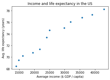
# This can make things like plotting this data a little easier (no need to filter ahead of time)
g = sns.scatterplot(x = gap_wide['gdpPercap']['United States'],
                    y = gap_wide['lifeExp']['United States']
                   )

g.set_xlabel("Average income ($ GDP / capita)")
g.set_ylabel("Avg. life expectancy (years)")
g.set_title("Income and life expectancy in the US")

Text(0.5, 1.0, 'Income and life expectancy in the US')

Bonus: `stack` and `unstack`¶

A really clear overview here

gap_stack = gap_wide.stack("country")

gap_stack
# gap_stack.columns

	measure	gdpPercap	lifeExp	pop
year	country
1952	Afghanistan	779.445314	28.801	8425333.0
	Albania	1601.056136	55.230	1282697.0
	Algeria	2449.008185	43.077	9279525.0
	Angola	3520.610273	30.015	4232095.0
	Argentina	5911.315053	62.485	17876956.0
...	...	...	...	...
2007	Vietnam	2441.576404	74.249	85262356.0
	West Bank and Gaza	3025.349798	73.422	4018332.0
	Yemen, Rep.	2280.769906	62.698	22211743.0
	Zambia	1271.211593	42.384	11746035.0
	Zimbabwe	469.709298	43.487	12311143.0

1704 rows × 3 columns

# gap_stack['pop']
# gap_stack[gap_stack['year'] == 2007]

gap_unstack = gap_stack.unstack("year")
gap_unstack

measure	gdpPercap										...	pop
year	1952	1957	1962	1967	1972	1977	1982	1987	1992	1997	...	1962	1967	1972	1977	1982	1987	1992	1997	2002	2007
country
Afghanistan	779.445314	820.853030	853.100710	836.197138	739.981106	786.113360	978.011439	852.395945	649.341395	635.341351	...	10267083.0	11537966.0	13079460.0	14880372.0	12881816.0	13867957.0	16317921.0	22227415.0	25268405.0	31889923.0
Albania	1601.056136	1942.284244	2312.888958	2760.196931	3313.422188	3533.003910	3630.880722	3738.932735	2497.437901	3193.054604	...	1728137.0	1984060.0	2263554.0	2509048.0	2780097.0	3075321.0	3326498.0	3428038.0	3508512.0	3600523.0
Algeria	2449.008185	3013.976023	2550.816880	3246.991771	4182.663766	4910.416756	5745.160213	5681.358539	5023.216647	4797.295051	...	11000948.0	12760499.0	14760787.0	17152804.0	20033753.0	23254956.0	26298373.0	29072015.0	31287142.0	33333216.0
Angola	3520.610273	3827.940465	4269.276742	5522.776375	5473.288005	3008.647355	2756.953672	2430.208311	2627.845685	2277.140884	...	4826015.0	5247469.0	5894858.0	6162675.0	7016384.0	7874230.0	8735988.0	9875024.0	10866106.0	12420476.0
Argentina	5911.315053	6856.856212	7133.166023	8052.953021	9443.038526	10079.026740	8997.897412	9139.671389	9308.418710	10967.281950	...	21283783.0	22934225.0	24779799.0	26983828.0	29341374.0	31620918.0	33958947.0	36203463.0	38331121.0	40301927.0
...	...	...	...	...	...	...	...	...	...	...	...	...	...	...	...	...	...	...	...	...	...
Vietnam	605.066492	676.285448	772.049160	637.123289	699.501644	713.537120	707.235786	820.799445	989.023149	1385.896769	...	33796140.0	39463910.0	44655014.0	50533506.0	56142181.0	62826491.0	69940728.0	76048996.0	80908147.0	85262356.0
West Bank and Gaza	1515.592329	1827.067742	2198.956312	2649.715007	3133.409277	3682.831494	4336.032082	5107.197384	6017.654756	7110.667619	...	1133134.0	1142636.0	1089572.0	1261091.0	1425876.0	1691210.0	2104779.0	2826046.0	3389578.0	4018332.0
Yemen, Rep.	781.717576	804.830455	825.623201	862.442146	1265.047031	1829.765177	1977.557010	1971.741538	1879.496673	2117.484526	...	6120081.0	6740785.0	7407075.0	8403990.0	9657618.0	11219340.0	13367997.0	15826497.0	18701257.0	22211743.0
Zambia	1147.388831	1311.956766	1452.725766	1777.077318	1773.498265	1588.688299	1408.678565	1213.315116	1210.884633	1071.353818	...	3421000.0	3900000.0	4506497.0	5216550.0	6100407.0	7272406.0	8381163.0	9417789.0	10595811.0	11746035.0
Zimbabwe	406.884115	518.764268	527.272182	569.795071	799.362176	685.587682	788.855041	706.157306	693.420786	792.449960	...	4277736.0	4995432.0	5861135.0	6642107.0	7636524.0	9216418.0	10704340.0	11404948.0	11926563.0	12311143.0

142 rows × 36 columns

UCSD CSS 2 - Spring 2022

Lecture 11 (4/20/2022)¶

Wide and Long Data¶

What is wide data?¶

So what’s the problem?¶

What do we do about this? Answer: tidy (long) data!¶

So what does tidy data do for us?¶

Pandas helps you convert data easily¶

Converting from wide to long with `melt`¶

Converting from long to wide with `pivot`¶

Bonus: `stack` and `unstack`¶

UCSD CSS 2 - Spring 2022

Lecture 11 (4/20/2022)¶

Wide and Long Data¶

What is wide data?¶

So what’s the problem?¶

What do we do about this? Answer: tidy (long) data!¶

So what does tidy data do for us?¶

Pandas helps you convert data easily¶

Converting from wide to long with melt¶

Converting from long to wide with pivot¶

Bonus: stack and unstack¶

Converting from wide to long with `melt`¶

Converting from long to wide with `pivot`¶

Bonus: `stack` and `unstack`¶