2022)¶

Announcements

Lab 5 may take a little longer than previous labs
Pset 3 due today
Purva’s OH in ERCA after lab today

Last time we covered:

Linear regression basics (ordinary least squares)

Today’s agenda:

Evaluating linear regression

import numpy as np
import pandas as pd
import matplotlib.pyplot as plt
import seaborn as sns

Deep Dive: regression in python¶

Last time, we talked about a number of different solutions for doing regression in python.

The most popular option, and the one we’ll focus on today, is the scikit LinearRegression class.

*Context: scikit is a robust set of tools for data science and analysis. Take a look at their other model-fitting resources here.

mpg = sns.load_dataset('mpg')

mpg

	mpg	cylinders	displacement	horsepower	weight	acceleration	model_year	origin	name
0	18.0	8	307.0	130.0	3504	12.0	70	usa	chevrolet chevelle malibu
1	15.0	8	350.0	165.0	3693	11.5	70	usa	buick skylark 320
2	18.0	8	318.0	150.0	3436	11.0	70	usa	plymouth satellite
3	16.0	8	304.0	150.0	3433	12.0	70	usa	amc rebel sst
4	17.0	8	302.0	140.0	3449	10.5	70	usa	ford torino
...	...	...	...	...	...	...	...	...	...
393	27.0	4	140.0	86.0	2790	15.6	82	usa	ford mustang gl
394	44.0	4	97.0	52.0	2130	24.6	82	europe	vw pickup
395	32.0	4	135.0	84.0	2295	11.6	82	usa	dodge rampage
396	28.0	4	120.0	79.0	2625	18.6	82	usa	ford ranger
397	31.0	4	119.0	82.0	2720	19.4	82	usa	chevy s-10

398 rows × 9 columns

# Let's look at the data
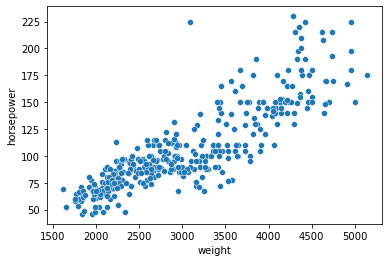
# Is there a linear relationship between "weight" and "horsepower"?

sns.scatterplot(data = mpg,
                x = "weight",
                y = "horsepower"
               )

<AxesSubplot:xlabel='weight', ylabel='horsepower'>

# Let's make sure this data is cleaned up by checking for null values!
# Handy resource: https://datatofish.com/rows-with-nan-pandas-dataframe/


mpg[mpg.isna().any(axis=1)]

# mpg.shape
# mpg.index

	mpg	cylinders	displacement	horsepower	weight	acceleration	model_year	origin	name
32	25.0	4	98.0	NaN	2046	19.0	71	usa	ford pinto
126	21.0	6	200.0	NaN	2875	17.0	74	usa	ford maverick
330	40.9	4	85.0	NaN	1835	17.3	80	europe	renault lecar deluxe
336	23.6	4	140.0	NaN	2905	14.3	80	usa	ford mustang cobra
354	34.5	4	100.0	NaN	2320	15.8	81	europe	renault 18i
374	23.0	4	151.0	NaN	3035	20.5	82	usa	amc concord dl

# Looks like we need to handle the null values above
mpg_clean = mpg.dropna().reset_index(drop = True)

mpg_clean[mpg_clean.isna().any(axis=1)]
# mpg.shape
# mpg.index

	mpg	cylinders	displacement	horsepower	weight	acceleration	model_year	origin	name

from sklearn.linear_model import LinearRegression # first, import the LinearRegression model class

# Prepare our data
x_vals = np.array(mpg_clean['weight'])
x_vals = x_vals.reshape(len(x_vals), 1) # what's going on here?
# x_vals[0]
# x_vals[0, 0]
# list(x_vals)
# x_vals
# TODO is there a more intuitive explanation for this?


y_vals = np.array(mpg_clean['horsepower'])


# Initialize the model
mod = LinearRegression()
# Fit the model
mod = mod.fit(X = x_vals, y = y_vals)

mod

LinearRegression()

Our (fitted) model comes with a number of attributes, including, most critically, the intercept and slope estimates

# Look at the values
mod.intercept_
# mod.coef_ # why is this different from the above?

# Other attributes we won't get into here

-12.1834847034594

Reminder: what do these values actually mean?

…

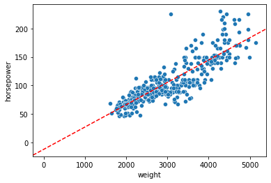
sns.scatterplot(data = mpg,
                x = "weight",
                y = "horsepower"
               )

plt.axline(xy1 = (0, mod.intercept_), slope = mod.coef_[0], color = "r", linestyle = "--")

<matplotlib.lines._AxLine at 0x7fd490edbb80>

Your turn!¶

Take a few minutes now to choose another pair of variables from this dataset.

Plot them to see if they have a linear(ish) relationship, then fit a regression to them and examine the parameter estimates.

NOTE: when doing this, try not to just copy-paste what I have above; instead, write it out yourself while looking back at the code when you need to.

Why? Copy-pasting is a big part of coding, but it works better when you’re already familiar with the syntax and just need the right details. When you’re doing something for the first time, it’s good to internalize what you’re doing!

### YOUR CODE HERE

What variables did you choose? How did your regression do?

weight / acceleration
weight / mpg

Above we looked at some of the attributes of our model class.

This class also has several useful functions. We’ve seen one already above (fit()).

What else can a LinearRegression object do?

# Other functions we can use

mod_preds = mod.predict(X = x_vals) # what is this doing?
# mod_preds

mod_score = mod.score(X = x_vals, y = y_vals) # what is this? 
mod_score

# These are the primary ones

0.74742549968982

Evaluating linear regression¶

In the section above, we generated a regression for the relationship between weight and horsepower.

How do we know if our regression is a good fit to the data? What gives you confidence that it’s describing the relationship between the variables well?

\(R^2\) (coefficient of determination): how much variance are we explaining?¶

\( R^2 = 1 - \dfrac{RSS}{TSS} \)

\( RSS = \sum_{i=1}^{n}{(y_i - \hat{y_i})}^2 \)

Where have we seen this before?

\( TSS = \sum_{i=1}^{n}{(y_i - \bar{y})}^2 \)

What does this look like?

\(R^2\) ranges between 0 and 1 and can be thought of as the percentage of variance in \(y\) that our model explains.

Intuition for this metric: divide the SS for our guess by the SS if our guess was just the mean of \(y\).

Raw value of RSS will vary depending on how many data points we have
What’s the lowest value that RSS could have? …
What’s the highest value that RSS could have? …

So our RSS should be somewhere between 0 (good) and whatever we would get from guessing \(\bar{y}\) for every point (bad). Divide RSS by that worst case value to indicate how close we are to worst case, then subtract from 1 for how close we are to best case.

Here’s a graphic illustrating it (source: wikipedia)

rsq

Let’s calculate it by hand so we understand it better:

rsq_mod = mod.score(X = x_vals, y = y_vals) # R^2 value
rsq_mod

# Add predicted y values to dataframe
preds = mod.predict(X = x_vals)
mpg_clean = mpg_clean.assign(model_pred = pd.Series([x for x in preds]))
mpg_clean

# Calculate RSS based on predicted values
mpg_clean = mpg_clean.assign(resid_sum_sq = (mpg_clean['horsepower'] - mpg_clean['model_pred'])**2)

# Calculate TSS based on mean of y
ybar = mpg_clean['horsepower'].mean()
mpg_clean = mpg_clean.assign(total_sum_sq = (mpg_clean['horsepower'] - ybar)**2)

rsq_hand = 1 - mpg_clean['resid_sum_sq'].sum() / mpg_clean['total_sum_sq'].sum()
rsq_hand

# What is the R^2 value?
print("Model value: {}".format(rsq_mod))
print("Hand calculation: {}".format(rsq_hand))

Model value: 0.74742549968982
Hand calculation: 0.74742549968982

Out of sample prediction (more on this later!)¶

Since the goal with our model is prediction, another way we can test whether it’s doing a good job is to see how it predicts new data!

There are a number of different approaches for this that we’ll talk more about later.

For now, let’s demonstrate a simple one: train the model, then test on hold-out data.

Step 1 is to randomly sample, e.g., 25% of our data and set it aside as the test data.

# Randomly sample 25% of our data points to be test data

from sklearn.model_selection import train_test_split

x_vals = np.array(mpg_clean['weight']).reshape(len(x_vals), 1)
y_vals = mpg_clean['horsepower']

xtrain, xtest, ytrain, ytest = train_test_split(x_vals, y_vals, 
                                                test_size = 0.25, 
                                                random_state = 1
                                               )


# mpg_clean.shape
# len(xtrain)

Step 2 is to fit our regression to the training data only.

# Initialize the model
mod_tr = LinearRegression()
# Fit the model
mod_tr = mod_tr.fit(X = xtrain, y = ytrain)

mod_tr.intercept_
mod_tr.coef_

array([0.03894649])

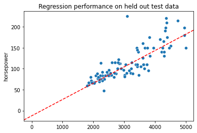
Step 3 is to see how well our regression model performs on the held out test data

mod_preds = mod_tr.predict(X = xtest)

mod_preds

array([ 85.08612203,  72.03904762,  79.01046947,  99.18475168,
        65.18446525,  68.30018451,  72.74008445, 152.50249753,
        76.59578704,  76.67368002, 113.8675787 ,  70.98749237,
       137.0407407 ,  63.23714071,  85.82610535, 121.81266281,
        79.78939928,  78.42627211, 157.05923695, 100.97629026,
        74.96003443, 128.93987062, 119.86533828, 149.6983502 ,
       156.55293257, 140.93538978,  67.13178978, 129.67985395,
       105.8446016 ,  80.37359664, 120.87794704,  94.19960086,
       162.82331759,  97.89951749, 120.87794704, 151.64567474,
       134.89868371, 125.16206102,  64.01607052,  70.4422415 ,
       155.92978872, 158.26657817,  96.80901574, 100.46998588,
        96.10797891, 132.75662672, 182.10183051,  64.21080298,
       113.40022081, 171.89784993, 130.49773025, 110.36239453,
        91.78491844,  76.86841247,  59.34249163, 103.70254461,
        88.5523597 ,  88.24078778,  87.03344656,  57.58989955,
       104.90988582,  83.45036941,  64.40553543, 118.54115759,
       107.63614018, 112.54339801, 114.84124097, 128.04410134,
        62.45821089, 180.4660779 ,  82.28197469, 127.88831537,
       133.73028899,  72.70113796,  74.49267654,  62.06874599,
       107.67508667, 161.34335094, 153.94351769,  84.46297817,
       128.47251273,  73.90847918,  66.11918102,  72.77903094,
       136.30075738, 120.48848213,  59.53722409,  91.47334651,
        63.43187316, 104.79304635,  71.76642219, 122.43580667,
       154.761394  , 158.14973869, 180.34923843,  92.64174123,
       154.72244751,  96.34165786])

sns.scatterplot(x = xtest.reshape(len(xtest)),
                y = ytest
               )

plt.axline(xy1 = (0, mod_tr.intercept_), slope = mod_tr.coef_[0], color = "r", linestyle = "--")

plt.title("Regression performance on held out test data")

Text(0.5, 1.0, 'Regression performance on held out test data')

Step 4 is …

… now what?

Let’s compare how our model did on the testing data compared to the training data it was fit to.

There are lots of ways to do this (incl. the \(R^2\) values we discussed above) and we’ll spend more time looking at some of them next week.

But one commoon approach worth highlighting is the mean squared error.

Mean squared error (MSE) is just the average of the squared residuals or squared error, the same stuff we’ve been dealing with from the beginning.

\( MSE = \dfrac{1}{n - 2} \sum_{i=1}^{n}{(y_i - \hat{y_i})}^2 = \dfrac{1}{n - 2} \sum_{i=1}^{n}{\epsilon_i}^2 \)

This tells you, on average, how close your model was to the true value across all the data points.

Why the \(n - 2\) here?

Let’s calculate it for our train and test datasets and compare them.

Do you think they’ll be similar?

# Training MSE

# Generate model predictions for the training data
train_pred = mod_tr.predict(X = xtrain)
# Calculate the squared error of these predictions
train_error = (ytrain - train_pred)**2
# Get the mean squared error
train_mse = train_error.sum() / (len(train_error) - 2)
train_mse

# Test MSE

# Generate model predictions for the test data (we did this above already)
test_pred = mod_tr.predict(X = xtest)
# Calculate the squared error of the test predictions
test_error = (ytest - test_pred)**2
# Get the mean squared error for test data
test_mse = test_error.sum() / (len(test_error) - 2)
test_mse

print("Training MSE: {} \n Test MSE: {}".format(train_mse, test_mse))

Training MSE: 332.72896851897474 
 Test MSE: 516.4390434210967

What do these results mean?

Is this a pretty good regression fit?

…

Parameter estimates¶

The criteria above are mostly concerned with whether we’re doing a good job predicting our \(y\) values with this model.

Notice this completely ignores the actual parameter estimates of the model!

In many cases, part of what we’re concerned with isn’t just how well we predict our data, but what kind of relationship our model estimates between \(x\) and \(y\).

How large or small is the slope?
How confident are we in the estimate?

This isn’t data we get directly from the LinearRegression class.

Instead, we can calculate by hand or use another model class like the statsmodels class we saw on Monday.

import statsmodels.formula.api as smf

results = smf.ols('horsepower ~ weight', data = mpg_clean).fit()
results.summary()

OLS Regression Results
Dep. Variable:	horsepower	R-squared:	0.747
Model:	OLS	Adj. R-squared:	0.747
Method:	Least Squares	F-statistic:	1154.
Date:	Tue, 14 Jun 2022	Prob (F-statistic):	1.36e-118
Time:	18:22:11	Log-Likelihood:	-1717.0
No. Observations:	392	AIC:	3438.
Df Residuals:	390	BIC:	3446.
Df Model:	1
Covariance Type:	nonrobust

	coef	std err	t	P>\|t\|	[0.025	0.975]
Intercept	-12.1835	3.570	-3.412	0.001	-19.203	-5.164
weight	0.0392	0.001	33.972	0.000	0.037	0.041

Omnibus:	83.255	Durbin-Watson:	1.014
Prob(Omnibus):	0.000	Jarque-Bera (JB):	312.937
Skew:	0.892	Prob(JB):	1.11e-68
Kurtosis:	6.997	Cond. No.	1.13e+04

Notes:
[1] Standard Errors assume that the covariance matrix of the errors is correctly specified.
[2] The condition number is large, 1.13e+04. This might indicate that there are
strong multicollinearity or other numerical problems.

What do we learn from the above?

Understanding the full output requires a more extensive statistics discussion than we’re going to have, but there are a few important take-aways:

The coefficient for weight (0.0392) has a small standard error (0.001) and a very narrow 95% confidence interval (0.037, 0.041) based on the observations here. This means we’re pretty certain about this slope estimate.
The \(t\) value for the slope (33.97) is extremely large, meaning we’re very confident that this slope value is significantly different from 0. In other words, there is a significant relationship between weight and horsepower in this data.

This is another way that we can evaluate our regression: the parameter estimates themselves tell us something useful and reasonably precise about the unerlying data.

Regression failures¶

Above we went through how to interpret and evaluate our regression.

In this case, we were estimating a linear slope in data that had a pretty strong linear relationship.

But what are the ways that this can break down?

…

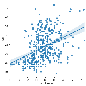
Noisy data¶

# mean = [0, 0]
# cov = [[1, 0], [0, 1]]
# x, y = np.random.multivariate_normal(mean, cov, 100).T


g = sns.scatterplot(data = mpg_clean, x = "acceleration", y = "mpg")

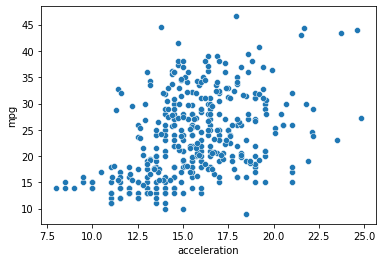
# Can we fit a regression to the data above?

m = LinearRegression().fit(
    X = np.array(mpg_clean['acceleration']).reshape(len(mpg_clean['acceleration']), 1), 
    y = np.array(mpg_clean['mpg'])
)

m.intercept_
m.coef_

m.score(
    X = np.array(mpg_clean['acceleration']).reshape(len(mpg_clean['acceleration']), 1), 
    y = np.array(mpg_clean['mpg'])
) 
# not so great...

0.1792070501562546

sns.lmplot(data = mpg_clean, x = "acceleration", y = "mpg")

<seaborn.axisgrid.FacetGrid at 0x7fd49194cfd0>

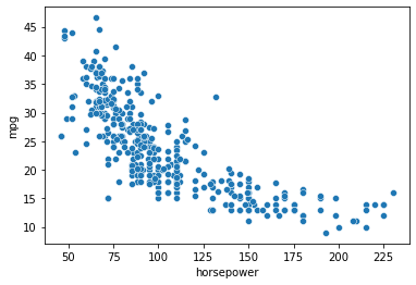
Non-linear data¶

# This doesn't seem like a linear relationship...

sns.scatterplot(data = mpg_clean, x = "horsepower", y = "mpg") # hp

<AxesSubplot:xlabel='horsepower', ylabel='mpg'>

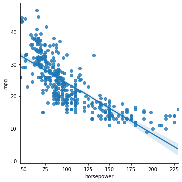
# Can we fit a regression to the data above?

m = LinearRegression().fit(
    X = np.array(mpg_clean['horsepower']).reshape(len(mpg_clean['horsepower']), 1), 
    y = np.array(mpg_clean['mpg'])
)

m.intercept_
m.coef_

m.score(
    X = np.array(mpg_clean['horsepower']).reshape(len(mpg_clean['horsepower']), 1), 
    y = np.array(mpg_clean['mpg'])
)

0.6059482578894348

sns.lmplot(data = mpg_clean, x = "horsepower", y = "mpg")

<seaborn.axisgrid.FacetGrid at 0x7fd4926cb0a0>

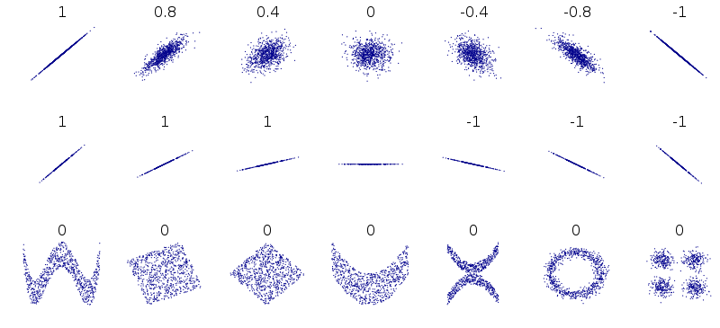
This graphic shows the correlation coefficient between two variables for a range of different data patterns.

The data that doesn’t have a strong correlation is also going to be difficult to fit a linear regression to.

corr_ex

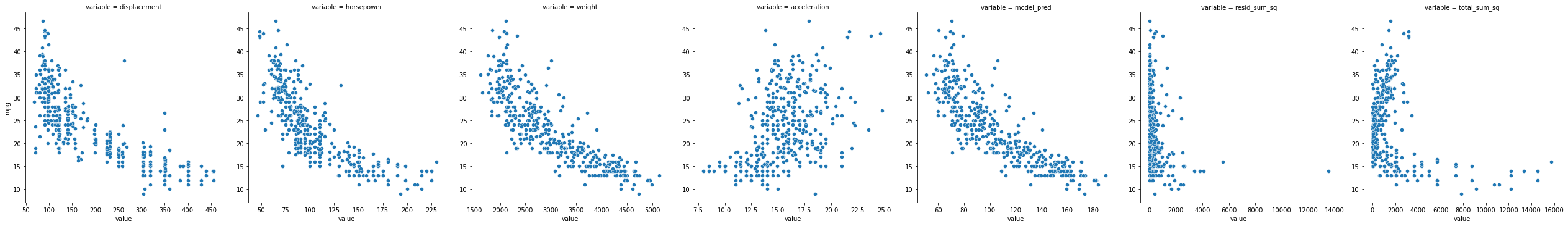
Multiple predictors¶

mpg_clean

mpg_long = mpg_clean.melt(
    id_vars = ["name", "origin", "model_year", "cylinders", "mpg"]
)
mpg_long

sns.relplot(data = mpg_long,
            x = "value",
            y = "mpg",
            col = "variable",
            kind = "scatter",
            facet_kws={'sharey': False, 'sharex': False}
           )

<seaborn.axisgrid.FacetGrid at 0x7fd4926c2ac0>

[next time] Failures of the linear regression assumptions¶

Ex. non-normal residuals

Lecture 13 (4/25/22) Lecture 15 (4/29/2022)

UCSD CSS 2 - Spring 2022